Reading and writing data

A short description of the post.

1. Load packages we will use.

library(tidyverse)
library(here)
library(janitor)
library(skimr)

2. Download \(CO_2\) emissions per capita from Our World in data into the directory of this post.

3. Assign the location of the file to file_csv. The data should be in the same directory as this file.

Read the data into R and read it as emissions

file_csv <- here("_posts",
                 "2021-03-01-reading-and-writing-data",
                 "co-emissions-per-capita.csv") 

emissions <- read_csv(file_csv)

4. Show the first 10 rows (observation of) emissions

emissions

# A tibble: 22,383 x 4
   Entity      Code   Year `Per capita CO2 emissions`
   <chr>       <chr> <dbl>                      <dbl>
 1 Afghanistan AFG    1949                    0.00191
 2 Afghanistan AFG    1950                    0.0109 
 3 Afghanistan AFG    1951                    0.0117 
 4 Afghanistan AFG    1952                    0.0115 
 5 Afghanistan AFG    1953                    0.0132 
 6 Afghanistan AFG    1954                    0.0130 
 7 Afghanistan AFG    1955                    0.0186 
 8 Afghanistan AFG    1956                    0.0218 
 9 Afghanistan AFG    1957                    0.0343 
10 Afghanistan AFG    1958                    0.0380 
# ... with 22,373 more rows

5. Start with emissions data THEN

use clean_names from the janitor package to make the names easier to work with assign the output to tidy_emissions show the first ten rows of tidy_emissions

tidy_emissions <- emissions %>% 
  clean_names()
tidy_emissions

# A tibble: 22,383 x 4
   entity      code   year per_capita_co2_emissions
   <chr>       <chr> <dbl>                    <dbl>
 1 Afghanistan AFG    1949                  0.00191
 2 Afghanistan AFG    1950                  0.0109 
 3 Afghanistan AFG    1951                  0.0117 
 4 Afghanistan AFG    1952                  0.0115 
 5 Afghanistan AFG    1953                  0.0132 
 6 Afghanistan AFG    1954                  0.0130 
 7 Afghanistan AFG    1955                  0.0186 
 8 Afghanistan AFG    1956                  0.0218 
 9 Afghanistan AFG    1957                  0.0343 
10 Afghanistan AFG    1958                  0.0380 
# ... with 22,373 more rows

6. Start with the tidy_emissions THEN use filter to extract rows with year==1993 THEN use skim to calculate the descriptive statistics.

tidy_emissions %>% 
  filter(year==1993) %>% 
  skim()

Table 1: Data summary

Name	Piped data
Number of rows	218
Number of columns	4
_______________________
Column type frequency:
character	2
numeric	2
________________________
Group variables	None

Variable type: character

skim_variable	n_missing	complete_rate	min	max	empty	n_unique	whitespace
entity	0	1.00	4	32	0	218	0
code	12	0.94	3	8	0	206	0

Variable type: numeric

skim_variable	n_missing	complete_rate	mean	sd	p0	p25	p50	p75	p100	hist
year	0	1	1993.00	0.00	1993.00	1993.00	1993.00	1993.00	1993.00	▁▁▇▁▁
per_capita_co2_emissions	0	1	4.97	6.83	0.04	0.55	2.57	7.25	61.85	▇▁▁▁▁

7. 12 observations have a missing code. How are these observations different? start with tidy_emissions then extract rows with year==1993 and are missing a code.

tidy_emissions %>% 
  filter(year==1993, is.na(code))

# A tibble: 12 x 4
   entity                     code   year per_capita_co2_emissions
   <chr>                      <chr> <dbl>                    <dbl>
 1 Africa                     <NA>   1993                     1.05
 2 Asia                       <NA>   1993                     2.21
 3 Asia (excl. China & India) <NA>   1993                     3.19
 4 EU-27                      <NA>   1993                     8.53
 5 EU-28                      <NA>   1993                     8.72
 6 Europe                     <NA>   1993                     9.36
 7 Europe (excl. EU-27)       <NA>   1993                    10.5 
 8 Europe (excl. EU-28)       <NA>   1993                    10.6 
 9 North America              <NA>   1993                    14.0 
10 North America (excl. USA)  <NA>   1993                     4.87
11 Oceania                    <NA>   1993                    11.4 
12 South America              <NA>   1993                     2.04

Entities that are not countries do not have country codes.

8. Start with tidy_emissions THEN use filter to extract rows with year==1993 and without missing codes THEN use select to drop the year variable THEN use rename to change the variable entity to country assign the output to emissions_1993

emissions_1993 <- tidy_emissions %>% 
  filter(year==1993, !is.na(code)) %>% 
  select(-year) %>% 
  rename(country=entity)

9. Which 15 countries have the highest per_capita_co2_emissions?

start with emission_1993 THEN use slice_max to extract the 15 rows with the highest per_capita_co2_emissions assign the output to max_15_emitters

max_15_emitters <- emissions_1993 %>% 
  slice_max(per_capita_co2_emissions, n=15)

10. Which 15 countries have the lowest per_capita_co2_emissions?

start with emissions_1993 THEN use slice_min to extract the 15 rows with the lowest values assign the output to min_15_emitters

min_15_emitters <- emissions_1993 %>% 
  slice_min(per_capita_co2_emissions, n=15)

11. Use the bind_rows to bind together the max_15_emitters and the min_15_emitters assign the output to max_min_15

max_min_15 <- bind_rows(max_15_emitters, min_15_emitters)

12. Export max_min_15 to 3 file formats

max_min_15 %>% write_csv("max_min_15.csv")#coma-separated values
max_min_15 %>% write_tsv("max_min_15.tsv")#tab-separated
max_min_15 %>% write_delim("max_min_15.psv", delim="|")#pipe separated

13. Read the 3 file formats into R

max_min_15_csv <- read_csv("max_min_15.csv")#coma-separated values
max_min_15_tsv <- read_tsv("max_min_15.tsv")#tab-separated
max_min_15_psv <- read_delim("max_min_15.psv", delim="|")#pipe separated

14. Use setdiff to check for any differences among max_min_15_csv, max_min_15_tsv and max_min_15_psv

setdiff(max_min_15_csv, max_min_15_tsv, max_min_15_psv)

# A tibble: 0 x 3
# ... with 3 variables: country <chr>, code <chr>,
#   per_capita_co2_emissions <dbl>

Are there any differences?

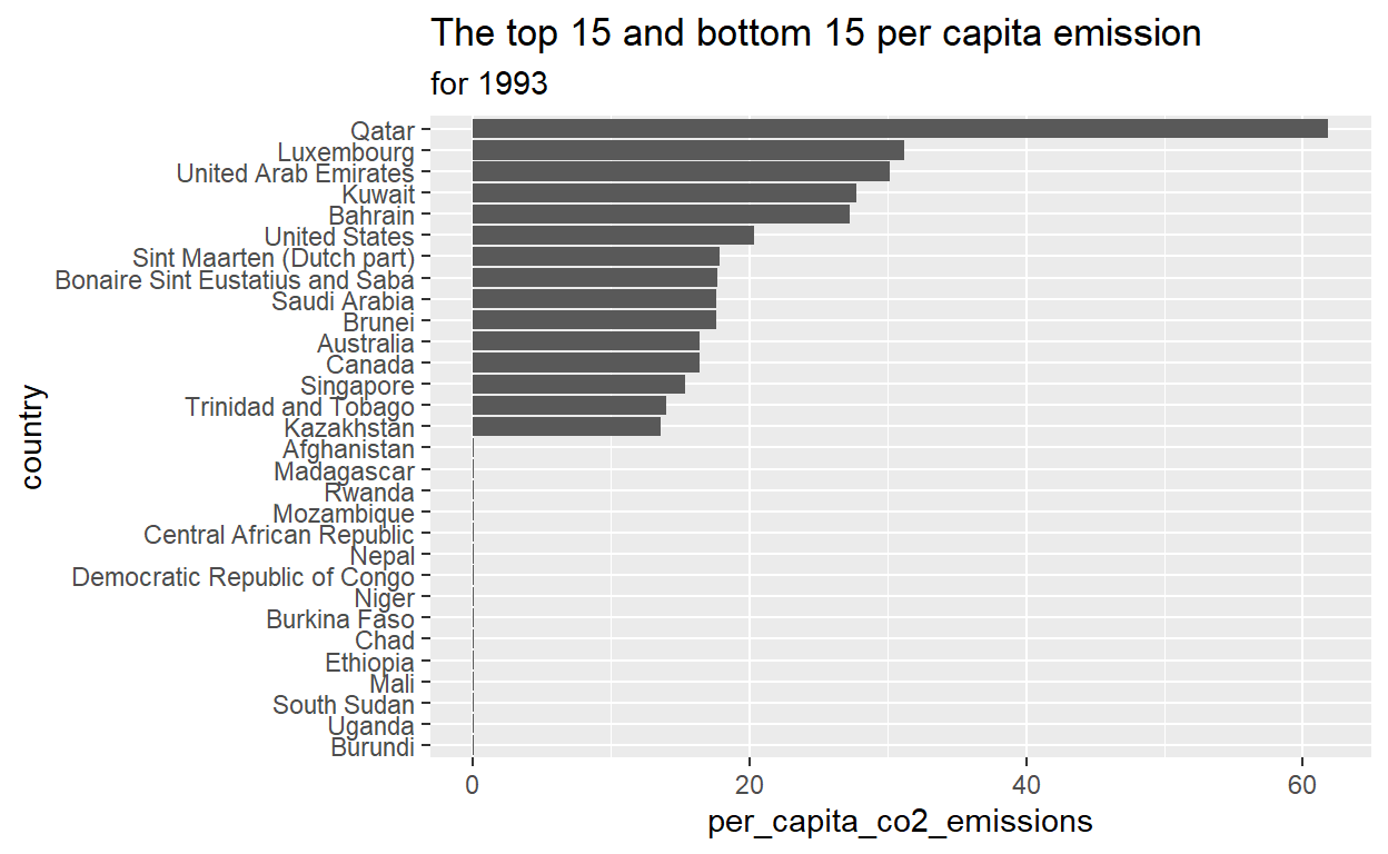
15. Reorder country in max_min_15for plotting and assign to max_min_15_plot_data

start with emissions_1993 THEN use mutate to reorder country according to per_capita_co2_emissions

max_min_15_plot_data <- max_min_15 %>% 
  mutate(country=reorder(country, per_capita_co2_emissions))

16. Plot max_min_15_plot_data

ggplot(data = max_min_15_plot_data, 
       mapping= aes(x=per_capita_co2_emissions, y=country))+
geom_col()+
labs(title = "The top 15 and bottom 15 per capita emission", subtitle = "for 1993")

x=NULL
y=NULL

19. Save the plot with this post.

ggsave(filename= "preview.png", path= here("_posts", "2021-03-01-reading-and-writing-data"))

18. Add preview.png to yaml chuck at the top of this file

preview: preview.png